Get in Touch with BBP

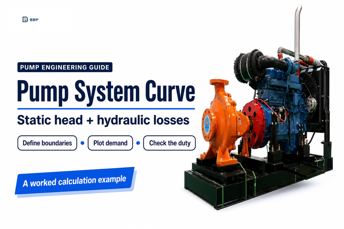
A pump system curve is a plot that shows the head required at each flow rate. In the case of a water-transfer line, this means that static demand is added to flow-dependent losses. A graph of this demand is compared to the pump performance curve to clarify the reasons for the changes in the quoted flow when the position of a valve changes or the level in a tank changes.
Updated September 2026
Quick reference
Model: Hsys = Hstatic + KsysQ². Example units: Q in m³/h; H in m of liquid. Scope: steady, single-phase flow through one liquid-filled series path. The numerical pump curve is illustrative, not a BBP product rating.
A pump system curve plots required head against flow. Static head sets the zero-flow intercept; hydraulic losses raise the curve as flow increases. The pump-curve intersection gives a candidate operating point that still needs operating-region and suction checks.
Key takeaways
- A curve intersection doesn’t automatically equal the best efficiency point.
- Static head includes boundary pressure as well as elevation.
- Closing a passive valve changes the system curve; changing speed changes the pump curve.
- Send a family of operating conditions with a quotation request when liquid levels or controls vary.
What Is a Pump System Curve?
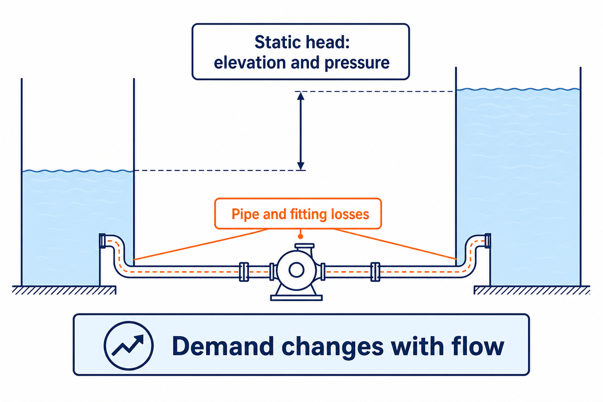
A pump system curve describes the variations in differential head required to move liquids through a given installation as the rate of flow changes. Head is plotted vertically against the rate of flow. The plots represent various conditions of the equipment and the routes taken by the liquids, and are made at various pressures and levels.
Head, measured in meters or feet, denotes the energy per unit weight of a liquid. One gauge reading alone doesn’t define the head. At a given pressure, the pressure head depends on the density or specific gravity of the fluid. In an installation, determine the total head and account for differences in readings from pressure gauges.
The Hydraulic Institute system-curve tutorial separates the static term from friction head, including major pipe losses and minor losses through fittings and equipment. “Minor” names a category; those losses can be a large part of a compact pump station’s demand.
“Static head consists of both the elevation and pressure difference between the supply and destination of the system.”
For the illustrative case of an open-tank line, 12 m of static head is remaining at zero flow. A purchaser of only “24 m duty” should enquire as to the tank levels and boundary pressures for this case. Otherwise, the supplier will be unable to distinguish static demand from the liquid head lost due to system friction.
Pump Curve vs System Curve: Find the Operating Point
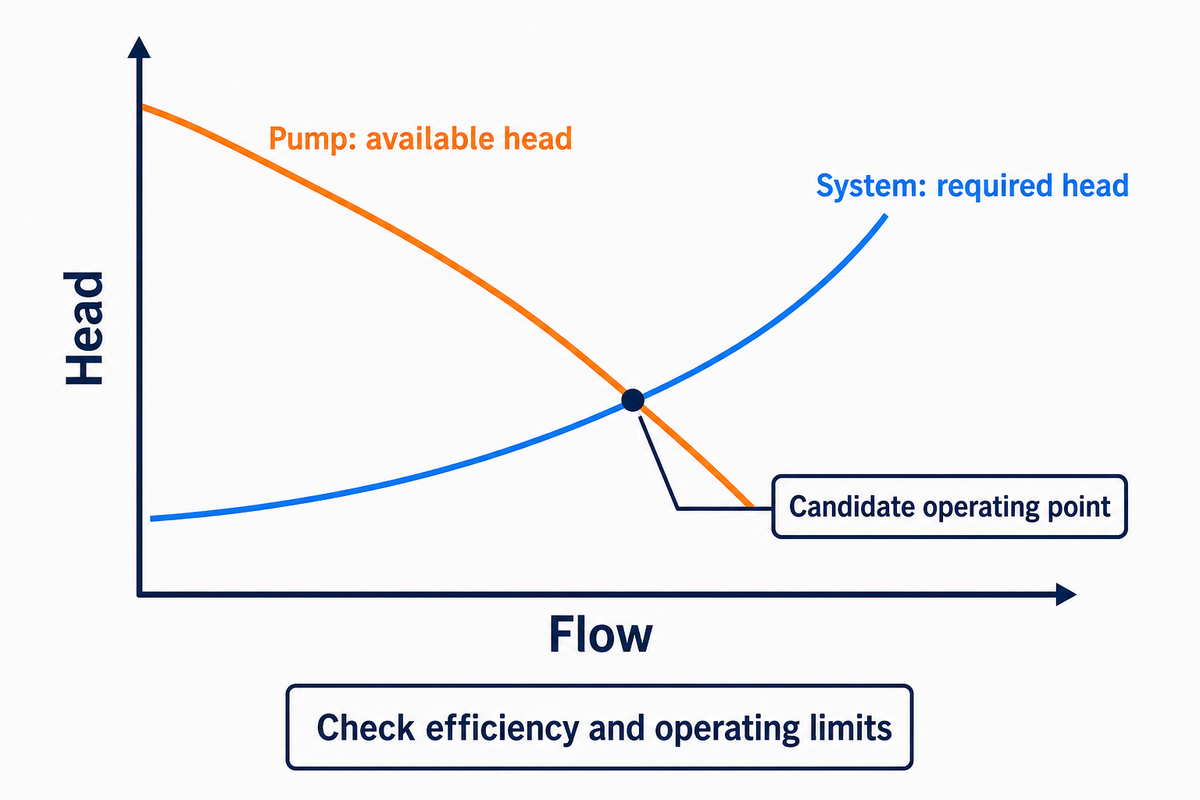
The pump curve is used to determine the available head at a specified speed and impeller diameter. The system curve shows required head. The intersection of the two lines indicates where the supplied and required heads are equal. The hydraulic equilibrium is an indication of a candidate duty point. This point should also be examined for level of effectiveness and for operation within limits.
What does a pump curve do?
A pump curve relates the head a pump can deliver to its flow under stated test conditions. A typical radial centrifugal pump has a generally descending head-flow characteristic over its working range. Manufacturer performance documents also show pump efficiency, absorbed power and suction requirements; one head-flow line can’t replace those separate quantities.
For information on characteristic curves and operating regions, see the Hydraulic Institute pump-curve guide. Best efficiency point (BEP) is the point of maximum pump efficiency and is shown on the pump curve diagram. The point of intersection may occur at a different location from BEP. Contact the supplier for the allowable and preferred operating regions for the pump type in question.
Let’s say a purchase is made specifying 49 m³/h at 24 m. Two suppliers may both meet this condition. Yet, differences in motor loading, allowed operating range and efficiency may occur. All these aspects must be analyzed in addition to price. Nominal flow and head don’t necessarily result in similar pump design or operating cost.
The example curves intersect at a flow rate of approximately 48.99 m³/h and a head of 24 meters. On their own, these two figures don’t allow determination of a Best Efficiency Point (BEP) and motor rating. Also, retain the manufacturer’s efficiency, power and suction curves with the quotation to ascertain the selected duty against the full performance data.
Build the System Curve from Static Head and Friction
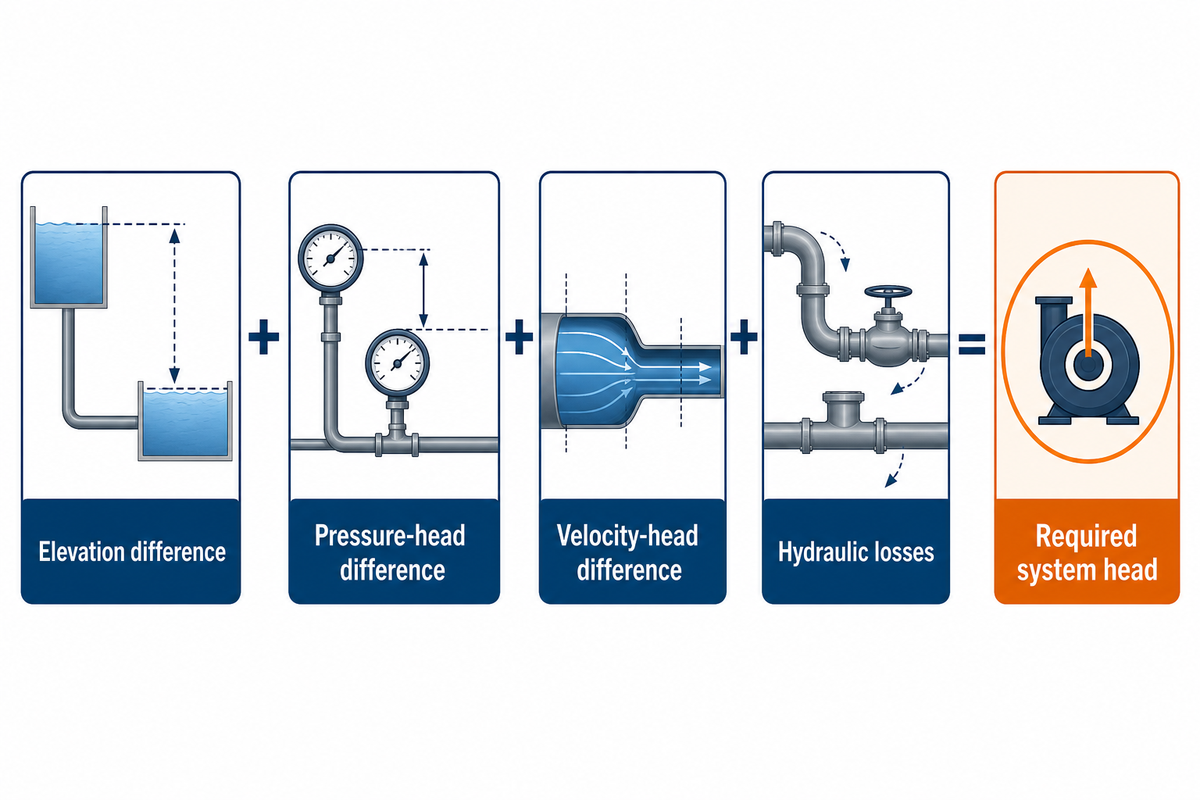
System-curve analysis relies on a balance of energy between two designated boundaries. Account for all kinds of differences in energy along the path, including friction losses. Calculate those losses using the energy equation. Perform the hydraulic calculations at various flows. In each of the analyses, keep all other conditions such as boundary conditions and positions of other valves constant.
Hsys(Q) = (z₂ − z₁) + (p₂ − p₁)/(ρg) + (v₂² − v₁²)/(2g) + ΣhL(Q)
This form uses SI units: pressure in Pa, density ρ in kg/m³, acceleration due to gravity g in m/s², velocity v in m/s, and elevation z in m. This simplified form assumes kinetic energy correction factors of approximately 1. For large reservoirs, the velocity may be negligibly small. Velocity at pressure taps in pipes, however, may be significant. It’s important to keep track of free surfaces. In the absence of proper corrections, it’s discouraged to mix free-surface and gauge boundaries.
The Darcy-Weisbach equation is straightforward. It states that hf = f(L/D)v²/(2g). Add fitting losses kLv²/(2g) and equipment losses using their applicable data. The Darcy friction factor is f. The length of the pipe is L and the internal pipe diameter is D. Generally, roughness and Reynolds number affect f.
When those resistance terms are approximately constant over the relevant turbulent-flow range, the pump system curve formula becomes Hsys = Hstatic + KsysQ². The system coefficient Ksys has units tied to Q; it’s different from a dimensionless fitting coefficient kL. Changing from m³/h to m³/s changes its numerical value.
9-Input Boundary-to-Curve Worksheet
The Boundary-to-Curve Worksheet identifies how each input is used in calculation and the evidence gaps the buyer must close.
| Input | Example or required record | Buyer action | Limitations / Not suitable for |
|---|---|---|---|
| Liquid and phase | Clean water, single phase | State temperature and properties | Slurry or gas entrainment needs separate treatment |
| Source boundary | Open-tank surface, z₁ = 0 m | Record minimum and maximum levels | One level cannot describe a cycling tank |
| Destination boundary | Open-tank surface, z₂ = 12 m | Use the same elevation datum | Highest pipe point is not automatically the endpoint |
| Boundary pressure | p₂ − p₁ = 0 Pa | Confirm both tanks vent to the same atmosphere | Pressurized vessels require pressure head |
| Endpoint velocity | Negligible at large tank surfaces | Identify boundary cross-sections | Finite-velocity gauge taps need correction |
| Static term | 12 m | Document elevation plus pressure calculation | Filled closed loops have different boundaries |
| Loss reference | 8 m at 40 m³/h | Replace assumed loss with calculated component data | One assumed point cannot validate field resistance |
| System coefficient | 0.005 m/(m³/h)² | Keep units beside the coefficient | Invalid if control state or resistance changes |
| Calculation range | 0–60 m³/h for the teaching plot | Check real model validity at each flow | Low-flow laminar behavior may depart from Q² |
Before accepting a quote, resolve whether the stated 8 m loss at 40 m³/h covers the entire series path, including inlet and discharge fittings. Omitting a strainer or short small-bore section changes the required head. The broader pump sizing calculation workflow helps assemble the remaining project inputs.
Worked Example: Plot Five Flows and Solve the Intersection
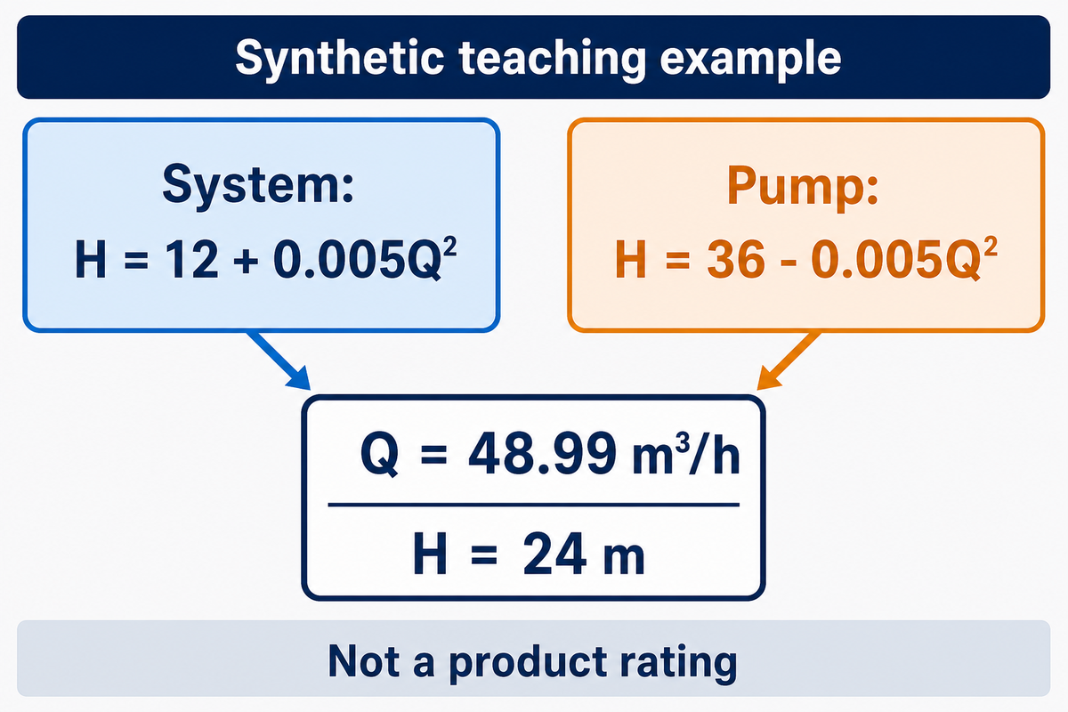
With 12 m static head and an assumed 8 m loss at 40 m³/h, the illustrative system equation is H sys = 12 + 0.005Q². Comparing it with the synthetic pump equation H p = 36 − 0.005Q² gives an intersection near 48.99 m³/h at 24 m.
Assume a plant engineer is reviewing an inter-unit water transfer and wishes to assess the calculation before including it in the request. The 8 m total head loss is assumed to be the net loss between the two surface impoundments. For the analysis, both surface water elevations are considered to be fixed. The engineer validates the shape and location of the intersection of Hp = 36 – 0.005Q2 and Hsys = 12 + 0.005Q2 and then replaces Hp with the data supplied by the manufacturer to evaluate the expectation for the pump.
- Set the boundaries. Use open surfaces separated by 12 m, with negligible surface velocity.
- Calculate resistance. Ksys = 8/40² = 0.005 m/(m³/h)².
- Calculate five points. Substitute Q = 0, 20, 40, 50 and 60 m³/h.
- Plot both series. Use flow on the horizontal axis and head on the vertical axis.
- Solve and qualify the duty. Equate the two heads, then check the manufacturer’s operating limits separately.
| Flow Q (m³/h) | Static head (m) | Loss (m) | System head (m) | Illustrative pump head (m) |
|---|---|---|---|---|
| 0 | 12 | 0 | 12 | 36 |
| 20 | 12 | 2 | 14 | 34 |
| 40 | 12 | 8 | 20 | 28 |
| 50 | 12 | 12.5 | 24.5 | 23.5 |
| 60 | 12 | 18 | 30 | 18 |
Therefore 24 = 0.010Q², Q = √2400 = 48.99 m³/h, and H = 12 + 0.005 × 2400 = 24 m. The Hydraulic Institute combined-curve tutorial explains the intersection method; the numerical inputs here are synthetic.
How do I calculate the pump curve?
A pump curve comes from a manufacturer’s performance data sheet or a controlled performance test, not an equation for system losses. For plotting, use the manufacturer’s data for flow and head at the specified speed and impeller diameter. The equation 36 − 0.005Q² is only a convenient teaching fit over this example’s 0–60 m³/h range.
In Excel, an XY scatter plot preserves the numerical spacing of the pump system curve chart. This isn’t necessarily the case with category line charts. Maintain units and stated limits beside the data to preserve the meaning of the plotted functions.
What Moves the Curve: Valves, Tank Levels, Speed, and Parallel Pumps
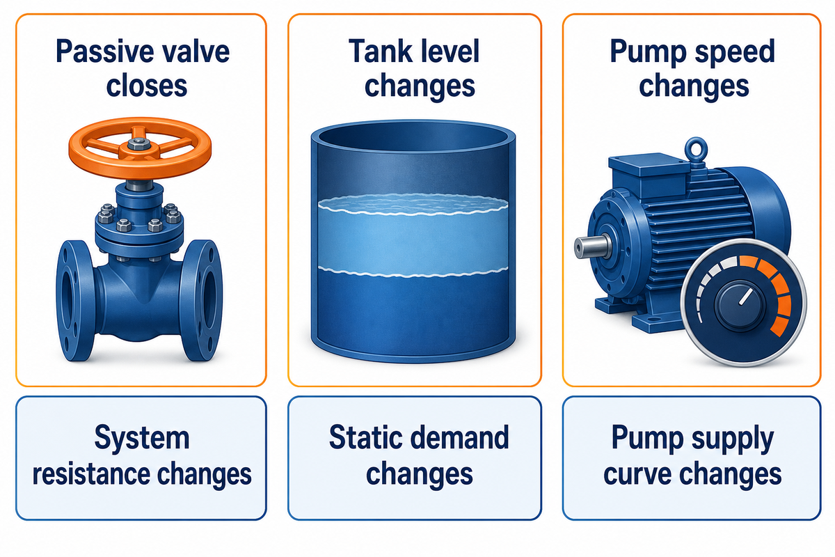
Resistance to flow increases when a fixed valve creates a greater flow restriction. A change in the level of fluid at an open-tank boundary changes the static term of the system. Likewise, a change in the speed of the pump changes the pump characteristic and its intersection with the system curve. Understanding the pump curve of the supply system allows for a logical explanation of the consequences of changes in system demand.
9-Case Curve-Shift Signature Table
The Curve-Shift Signature Table provides a logical framework for identifying and articulating the next information request.
| Change type | Curve effect | Decision or example | Limitations / Not suitable for |
|---|---|---|---|
| Discharge valve throttled | System resistance increases | Total K = 0.010 gives 40 m³/h at 28 m | Assumes passive fixed valve position |
| Destination level rises 6 m | Static intercept becomes 18 m | 42.43 m³/h at 27 m | Other boundary pressures held constant |
| Speed reduced to 80% | Pump curve shifts downward | 33.23 m³/h at 17.52 m | Affinity assumptions; unchanged passive system |
| Flow-control valve regulates | Valve loss adjusts with control action | Flow may remain at its setpoint | A single fixed-K curve may not describe operation |
| Strainer accumulates debris | Equipment loss increases | Compare differential pressure at comparable flow | Do not infer fouling from discharge pressure alone |
| Pipe internal diameter changes | Velocity and friction loss change | Recalculate the affected section | Nominal size alone does not establish bore |
| Parallel pump starts | Combine pump flows at equal head | Solve the new supply/system intersection | Do not assume double the flow; check entry conditions |
| Impeller diameter changes | Pump performance changes | Request the corresponding manufacturer curve | Speed affinity scaling is not an exact trimming rule |
| Branch demand changes | Network distribution changes | Check branch pressures and flows | Total flow alone cannot prove branch service |
The tutorial available at the Hydraulic Institute explains, by example, that an actively controlled valve can constrain flow. Use the affinity laws to calculate a variable speed pump curve for a fixed impeller: Hnew(Q) = r²Hold(Q/r). At a relative speed of 0.8, the pump would be expressed as 23.04 – 0.005Q². Equating it with the original system gives Q² = 1104, rather than simply taking 80% of the original duty flow.
Throttling in this example reduces flow from 48.99 m³/h to 40 m³/h while raising pump head from 24 m to 28 m. This change isn’t sufficient to conclude that the pump uses more or less power. Use the manufacturer’s pump power data and the pump power formula with efficiency to draw conclusions about motor loading and power consumption.
There are a few more things to check with parallel pumps. One pump can create a condition (or header) that another unit can’t satisfy. One example of this is the check-valve entry issue that occurs with stable and unstable pump curves, which is described in Lev Nelik’s technical discussion of stable and unstable pump curves. The supplier should be asked to validate the combination and starting sequence of the pumps provided, as a combined steady-state condition of the pumps doesn’t ensure that all the transient conditions are satisfied.
Check the Limits of the Quadratic Model
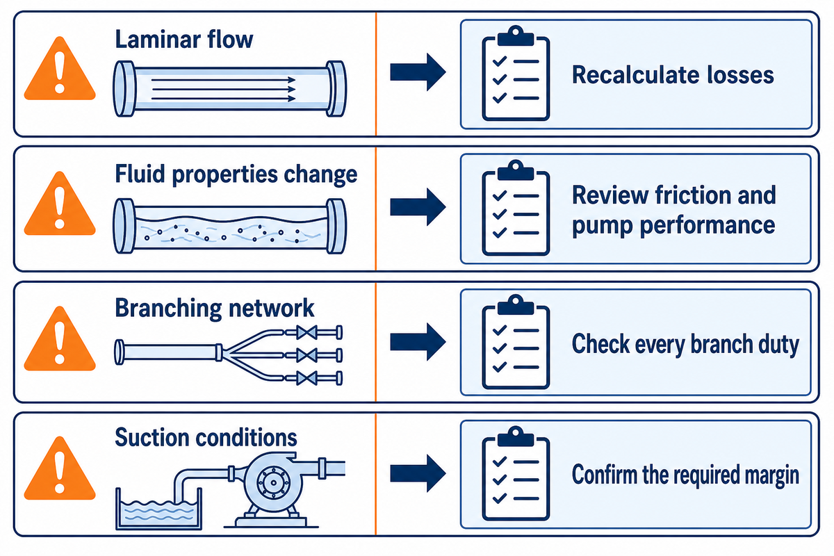
A quadratic model may be applied to a liquid-filled series path with pipe and minor losses, provided the loss coefficients and boundaries remain approximately constant. Laminar flow, changing fluid properties, branching piping systems and active controls may violate these assumptions and require recalculation of losses.
At low Reynolds number, straight-pipe loss doesn’t follow the same constant-f Q² relationship. Viscosity changes also affect friction and pump performance. Applying a clean-water curve directly to slurry pump selection omits the relevant hydraulic and material corrections.
In a filled closed loop returning to the same hydraulic boundary, the net static elevation term can be 0 m even when the pipe climbs uphill. Conditions of fill, including suction and pressure, may vary throughout the system. Just because a closed system reaches a particular elevation, that elevation doesn’t necessarily set the static head; local pressure and conditions of fill still need to be considered.
When not to select a pump from this example
Non-monotonic behavior of a pump can allow multiple candidate flows. Intersecting lines don’t guarantee a stable flow state. Request a supplier’s assessment to determine if the operating conditions of the flow system are within the supplier’s defined design limits. For branching piping systems, determine the flow and pressure required at each branch. A single path system doesn’t allow analysis of how the flow is distributed between the users.
There are independent limits set by conditions of suction, e.g. vacuum level. The Hydraulic Institute’s analysis describes factors impacting operating region and suction head. Available net positive suction head (NPSHA) equal to the manufacturer’s NPSH3 already corresponds to cavitation-related head reduction. It’s best to review case-by-case a given situation and assess if sufficient margin is available to support the manufacturer’s recommendation.
There’s uncertainty regarding suction performance at 48.99 m³/h for the teaching line. Don’t speculate with a presumed suction margin based on an arbitrary percentage of the best efficiency point (BEP). Wait on the manufacturer to verify the operable condition.
Use a Duty Envelope for Pump Selection and Quotations

A service envelope uses system head curves to define the range of head and flow over varying operating
conditions. With suction conditions and relevant fluid properties, potential customers
can ask the supplier to confirm the pump’s power and limits of operation. This allows the supplier
to evaluate the pump’s service and limits, rather than assess a single, nominal
value.
4-State Duty-Envelope Handoff Sheet
The Duty Envelope Handoff form identifies the evidence of acceptance still needed for various conditions before the specifying party can compare offers.
| Operating state | Candidate duty | Suction evidence to attach | Supplier confirmation |
|---|---|---|---|
| Base: static 12 m, K = 0.005 | 48.99 m³/h; 24 m | Source level, pressure, temperature and inlet losses | Operating region, efficiency and power at this duty |
| Throttled: total K = 0.010 | 40 m³/h; 28 m | Recalculate inlet loss at reduced flow | Permitted continuous operation and valve/control arrangement |
| Higher destination: static 18 m | 42.43 m³/h; 27 m | Confirm the source condition has not also changed | Coverage of this higher-head state |
| 80% speed; original system | 33.23 m³/h; 17.52 m | Available suction head at this state | Speed-specific curve, suction requirement and motor limits |
Which Supplier Curve Evidence Should You Request?
Request a performance curve from the service provider that identifies the limits of acceptance for the pump duty (continuous or intermittent) and defines any excluded combination of conditions. Ask the service provider to identify assumptions made for the analyzed liquid. Request a dated curve for the offered model, impeller diameter and speed, with efficiency, absorbed power and suction requirements at minimum, normal and maximum duties.
The public scope of ANSI/HI 9.6.3-2024 distinguishes
preferred and allowable operating regions. Limits for a centrifugal pump depend on design and the conditions of service; a
generic percentage band alone is insufficient to define those limits.
Suppose the operations team needs the unit running at base load the greater part of the day, and the maintenance team needs it at a throttled state during a process change. Finance receives a cheaper quotation that documents only 49 m³/h at 24 m. The handoff sheet exposes the missing 40 m³/h, 28 m assessment. The maintenance team should request the confirmation of the flow before shopping for the best price. The finance team also should request the consumption of power and the number of hours the unit is run in the various states, and head alone shouldn’t be the sole determinant for comparing the various alternatives. This approach ensures that the commercial decision made is for the service the unit will actually provide.
Complete the enclosed form when reviewing BBP centrifugal pump alternatives for a water transport service. Identify the expected flow of the service, and the properties of the liquid to be transported. Upon identification of a preliminary product, request specifics of the curve from the vendor.
From a Design Curve to an Operating Baseline
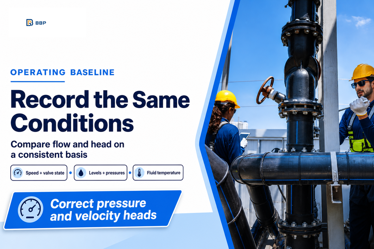
A baselined operation shows flow and head in the same condition. In the absence of such records, it may not be possible to differentiate between a change in operating conditions and a change in resistance. Useful information for curve analysis may be found in a number of operating condition changes.
When conditions warrant, record the date, flow, speed, suction and discharge readings, valve positions, gauge elevations and fluid temperature. Convert pressure readings to head using the relevant density and account for differing velocity heads where needed. Jim Elsey’s off-curve guidance may be of service.
If a team measures a flow rate of 40 m³/h after previously measuring a flow rate of 49 m³/h, the team must check the valve positions, the levels in the surge tanks, the differential pressure across the strainers and the baseline value. The example that reaches a flow rate of 40 m³/h does so because of increased resistance. This example doesn’t diagnose the process, but it gives a different explanation to check when the flow rate has decreased, before assuming impeller wear is the cause.
Key takeaway
A system curve supports a buying decision when its boundaries, units and operating states are documented. Pair each duty with manufacturer limits and suction evidence before accepting the pump selection.
To initiate a review of a pump based on the input you provided, send flow and liquid data to BBP via the online form in the BBP pump inquiry form.
Frequently Asked Questions
What is a system curve for a pump?
Read the answer
A system curve plots the head required by an installation against flow rate. Its shape depends on boundary pressures, liquid elevations and hydraulic losses through the selected flow path. For a simple fixed turbulent-flow system, static head supplies the intercept and an approximately flow-squared loss term supplies the rising portion. The assumptions must remain attached to the plotted line.
What is the difference between a system curve and a pump performance curve?
Read the answer
The system curve describes the installation’s demand, while the pump performance curve describes the head the pump can supply at a specified speed and impeller diameter. Changing pipe resistance moves the system curve. Changing pump speed moves the pump curve. Their intersection gives the hydraulic duty point for that particular combination, rather than automatically identifying the best efficiency point.
How is the system curve derived?
Read the answer
Start with the steady-flow energy balance between two defined boundaries. Include their elevation difference, pressure-head difference, any endpoint velocity-head difference, and all intervening hydraulic losses. For a fixed turbulent-flow installation, losses may be approximated as proportional to flow squared. Calculate several flow-and-head pairs using consistent units, then plot them. Recalculate when levels, valves, fluid properties or network paths change.
Does a system curve always start at zero?
Read the answer
No. A nonzero static head produces a nonzero intercept. A simple filled closed loop may have zero net static lift.
Can I build a pump system curve in Excel?
Read the answer
Yes. Put flow values in one column and calculated system head in another, then insert an XY scatter chart. For the illustrative equation in this article, enter =12+0.005*A2^2 when A2 contains flow in cubic metres per hour. Keep the units and assumptions next to the cells. Add a separate series using the manufacturer’s actual pump data; don’t treat the article’s illustrative pump equation as a product curve. Check that the chosen operating point lies within the supplier’s accepted range and that suction conditions have been assessed independently.
Does the operating point have to be at the best efficiency point?
Read the answer
No. The intersection follows the system demand and available pump head. Compare it with the manufacturer’s recommended operating region; don’t assume every intersection is acceptable.
Editorial note: This guide has been developed by BBP as a pump supplier. Some limitations of the models used in this guide are described in the sources below. All worked-example values are synthetic teaching inputs; they aren’t test results, a customer installation or a rating for any offered pump.
References & Sources
- System Curves, Hydraulic Institute.
- Pump Curves, Hydraulic Institute.
- Combined Pump & System Curves, Hydraulic Institute.
- Stable and Unstable Pump Curves, Lev Nelik, Pumps & Systems, 2011. Physical behavior discussion; dated standards quotations aren’t adopted.
- The Basics of NPSH & Pump Operating Regions, Peter Gaydon, Hydraulic Institute, 2022 republication. Terminology and physical principles; older cited editions aren’t presented as current.
- ANSI/HI 9.6.3-2024: Rotodynamic Pumps Guideline for Operating Regions, Hydraulic Institute, public scope.
- Why Is Your Pump Operating Off Its Curve?, Jim Elsey, Pumps & Systems, 2019.